Overview Link to heading
Goal: Explain how multilayer perceptron model is trained. Mostly for me to understand the foundation.
Half of the battle is the configurations and notations:
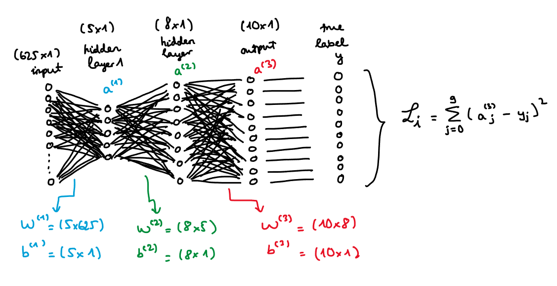
- Suppose we want to classify 25x25 images and have 10 output labels $(\textbf{y})$. The data for training are labeled and cleaned.
- There are $m$ instances in the data, 625 features, and 10 labels.
- The data can be represented as a $m \times 625$ matrix or tabular-type. For simplicity, we will work with each single training example (i.e. some $x_0$). That is, the input layer is a $1 \times 625$. As a convention (I believe), we should transpose this matrix and get the $625 \times 1$ input layer. Then, the output layer is the activations of 10 labels which is a $10 \times 1$ matrix. Output layer notation: $\textbf{a}^{(3)} = [ [a_0^{(3)}], [a_1^{(3)}], \ldots, [a_{9}^{(3)}]]$. To be more general, let $j$ index the output matrix’s elements.
- Choose 2 hidden layers: the first layer has 5 neurons and uses ReLU as the activation function and the second layer has 8 neurons and uses a softmax function. The number of neurons is arbitrarily selected. Respective layer notations: $\textbf{a}^{(1)} = [[a_0^{(1)}], [a_1^{(1)}], \ldots, [a_4^{(1)}]]$ and $\textbf{a}^{(2)} = [[a_0^{(2)}], [a_1^{(2)}], \ldots, [a_7^{(2)} ]]$. To be more general, let $k$ index the layer (2) matrix’s elements and let $h$ index the layer (1) matrix’s elements.
- Choose the Mean Squared Error (MSE) loss function. For one single training example $x_i$, $ℒ_i = \sum_{j=0}^{9} (a_j^{(3)} - y_j)^{2}$. Then, the overall loss function for all training examples is $ℒ = \frac{1}{m} \sum_{i=0}^{m-1} \mathscr{L_i}$.
- Choose the Stochastic Gradient Descent technique for mini-batching and randomization optimization. Iterate through each training example (or randomly selected mini-batches of examples) and compute the gradient of the loss function with respect to the $W$ and $b$ parameters using that example or mini-batch. Update the parameters with the computed gradients and a learning rate. Repeat the process for multiple iterations (epochs) until convergence or a stopping criterion is met.
- Last but not least: weight and bias parameters. They appear in each of the layers except for input layer.
- $\textbf{W}^{(1)}$ and $\textbf{b}^{(1)}$ denote the weights and biases of layer (1) in which $\textbf{W}^{(1)}$ is a $5 \times 625$ matrix and $\textbf{b}^{(1)}$ is a $5 \times 1$ matrix.
- $\textbf{W}^{(2)}$ and $\textbf{b}^{(2)}$ denote the weights and biases of layer (2) in which $\textbf{W}^{(2)}$ is a $8 \times 5$ matrix and $\textbf{b}^{(2)}$ is a $8 \times 1$ matrix.
- $\textbf{W}^{(3)}$ and $\textbf{b}^{(3)}$ denote the weights and biases of output layer in which $\textbf{W}^{(3)}$ is a $10 \times 8$ matrix and $\textbf{b}^{(3)}$ is a $10 \times 1$ matrix.
This is my attempt to draw a neural network for one single training example:
Additional notations Link to heading
- Weighted sum $z$ or linear combination of weights and activations along with bias, i.e. for layer $i$, $z^{(i)} = W^{(i)} a^{(i-1)} + b^{(i)}$.
- ReLU and softmax. MLP is inherently a linear model and we apply non-linear activation function.
- Why? (1) Nonlinear activation functions allow the network to stack layers and build a hierarchy of features. Each layer can learn different levels of abstraction, where higher layers build upon the outputs of lower layers. (2) The Universal Approximation Theorem states that a feedforward neural network with at least one hidden layer and a nonlinear activation function can approximate any continuous function to any desired degree of accuracy, given sufficient neurons in the hidden layer. (3) Nonlinear functions ensure that the gradients are non-zero and propagate through the network layers. This gradient back propagation is critical for learning, as it updates the weights based on the error evaluation.
- Why ReLU and softmax? Arbitrary for now. I think I need to dig deeper into the comparisons and criteria for choosing. In the softmax, $j$ in the index of the weighted sum $j$ in the vector $\textbf{z}^{(i)}$ of layer $i$, then take this exponentially and divided by the total sum of exponential weighted sum across the $\textbf{z}^{(i)}$ vector, then we get the logit probability. So, softmax is a vector of logit probabilities.
$$ \text{softmax}(z_j^{(i)}) = \frac{e^{z_j^{(i)}}}{\sum_{k=1}^{n} e^{z^{(i)}_k}} $$
$$ \text{ReLU}(z^{(i)}_j) = \max(0, z^{(i)}_j) $$
- Stochastic gradient descent (SGD), regularization. SGD is essentially the learning ($\eta$) after we get the gradients from back prop and update the weights and biases per layer. Regularization helps avoid overfitting. Here we arbitrarily use L2. More on this.
Algorithms Link to heading
Feed forward Link to heading
Suppose your network has $L$ layers. Make prediction for an instance $ \mathbf{x} $
- Initialize $ \mathbf{a}^0 = \mathbf{x} $ \hfill $ (\mathbf{d} \times 1) $
- For $ l = 1 $ to $L $ do
- $ \mathbf{z}^l = \mathbf{W}^l \mathbf{a}^{l-1} + \mathbf{b}^l $
- $ \mathbf{a}^l = g(\mathbf{z}^l) $
- The prediction $ \hat{y} $ is simply $ \mathbf{a}^L $
Back prop Link to heading
Back propagation is how we update weights for neural networks. Define $ \delta^l = \frac{\partial \mathcal{L}}{\partial \mathbf{z}^l} $
- Compute $ \delta $’s on output layer: $ \delta^L = \frac{\partial \mathcal{L}}{\partial \mathbf{a}^L} \circ g’^L (\mathbf{z}^L) $
- For $ l = L, \ldots, 1 $ do
- Compute bias derivatives: $ \frac{\partial \mathcal{L}}{\partial \mathbf{b}^l} = \delta^l $
- Compute weight derivatives: $ \frac{\partial \mathcal{L}}{\partial \mathbf{W}^l} = \delta^l (\mathbf{a}^{l-1})^T $
- Backprop $ \delta $’s to previous layer: $ \delta^{l-1} = (\mathbf{W}^l)^T \delta^l \circ g’^{l-1} (\mathbf{z}^{l-1}) $
The symbol $ \circ $ indicates element-wise multiplication of vectors.
SGD Link to heading
Hyperparameter: step size (learning rate) $ \eta $
- Initialize all parameters (which we will return to later)
- For $ t = 1, \ldots, T $ do
- Randomly shuffle the training data
- For each example $ x_i, y_i $ in training data do
- For $ l = 1, \ldots, L $ do
- Set $\mathbf{b}^l = \mathbf{b}^l - \eta (\frac{\partial \mathcal{L}}{\partial \mathbf{b}^l} + \lambda \frac{\partial \mathcal{L}}{\partial \mathbf{b}^l})$
- Set $ \mathbf{W}^l = \mathbf{W}^l - \eta (\frac{\partial \mathcal{L}}{\partial \mathbf{W}^l} + \lambda \frac{\partial \mathcal{L}}{\partial \mathbf{W}^l})$
- For $ l = 1, \ldots, L $ do
Output the parameters (each layer has a matrix of weight params and a vector of bias params).
Questions (to be answered) Link to heading
- How does the backprop really work? (Chain rule and lots of derivatives)
- Why do we use hidden layers?
- How can we determine the number of neurons per layers? And how many layers? In what kind of general context?
- Relationship between number of neurons/dimension per layer and model’s performance?
- Interpretability and intuition challenges.
- What loss function should we choose? In what case?
- What activation function in each layer? And why? In what context?
- How do we compare and make decision on what optimization technique to use?
- Backprop can cause vanishing gradients. Why?
- Are initial weights and biases chosen randomly? What is the advice?
Practice later: Heart disease classification Link to heading
Information on the data here .
# libraries
import pandas as pd
import numpy as np
from ucimlrepo import fetch_ucirepo

# fetch dataset
heart_disease = fetch_ucirepo(id=45)

# data (as pandas dataframes)
X = heart_disease.data.features
y = heart_disease.data.targets

# variable information
heart_disease.variables
References: Link to heading
Janosi,Andras, Steinbrunn,William, Pfisterer,Matthias, and Detrano,Robert. (1988). Heart Disease. UCI Machine Learning Repository. https://doi.org/10.24432/C52P4X .